How to Create a Work Schedule in Excel

Build a proper employee work schedule in Excel — one that calculates end times,
counts staff per day, totals hours, and highlights days off automatically.

We start from a blank sheet and build the whole thing. Beginner-friendly
throughout, with some formatting tricks near the end that make it look like a
real rota rather than a spreadsheet.

Watch: build the schedule in 12 minutes

Prefer reading? The same steps are written out below the video.

Step-by-step

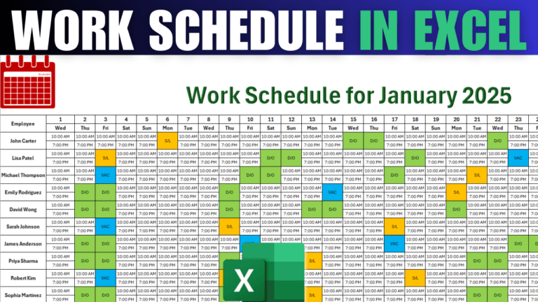
You’ll build a monthly staff schedule with start and finish times, days off, vacation and sick leave in colour, and automatic counts of staff per day and hours per person.

1. Fill in the days of the month

In a blank sheet, type 1 in B8 and select it again. Go to Home > Fill > Series, choose Rows and enter 31 as the stop value (January has 31 days). Excel fills in every day.

2. Make the columns narrow and add weekdays

Select the whole sheet and drag any column border to make the columns narrow and even. Under the 1, type the weekday the month starts on (for January 2025, Wed) and drag the fill handle across. Excel repeats the weekdays in order. Centre everything.

3. Add the employee rows

Each employee gets two rows: one for the start time and one for the finish time. Merge A8:A9 with Merge & Center, then use the fill handle to merge the pairs below. Type the column title and the employee names, widen the column and turn on Wrap Text. In the last row type Total number of employees per day. Select the table and apply All Borders.

4. Enter start times and calculate finish times

Type the first start time, for example 10:00 AM, in B10. Set the font to 10 and a time format. In the cell below (B11), add nine hours (eight hours of work plus a one-hour lunch):

=B10+TIME(9,0,0)

Depending on your regional settings you may need semicolons instead of commas. Copy both cells across to the other working days.

5. Mark days off, vacation and sick leave

For a day off, merge the two cells for that day and type D/O. Use V for vacation and SL for sick leave the same way. Fill in the rest of the staff.

6. Colour-code them

Select the time area (B10:AF29). Go to Conditional Formatting > New Rule > Format only cells that contain, choose Specific Text, type D/O and pick a green fill. Repeat for V (blue) and SL (orange). New entries colour themselves.

7. Count staff working each day

Merge the two cells in B30 and enter:

=COUNT(B10:B29)/2

COUNT only counts numbers, so D/O, V and SL are ignored. Dividing by two is needed because each working employee has two time cells. Drag the formula across the row.

8. Total hours per employee

Add a Total hours per employee column at the end. For the first employee, count their shifts and multiply by eight hours:

=COUNT(B10:AF11)/2*8

Copy it down for each employee.

9. Finish it off

Leave space at the top for a logo, title and a colour key. Then turn off gridlines from the View tab so the schedule is easier to read.

Go further

My Excel Tips & Shortcuts: 100+ Powerful Hacks course collects a hundred time-saving techniques like this one.