
THE DASHBOARD PACK
Kanban board, habit tracker, KPI report, search bar and more — built, working, ready to take apart. Free, instant, yours to keep.
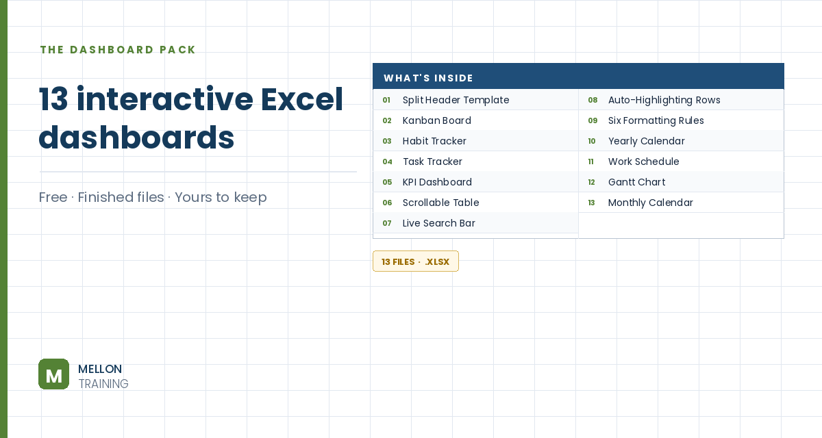
What’s in the pack
Free, instant, and yours to keep.
No spam, ever. Unsubscribe with one click.
One practical Excel tip a week.
Watch the 21-minute build or follow the main stages below. The free dashboard pack above has ten more finished dashboards to learn from.
You’ll build a sales dashboard where each product gets a traffic light (red, yellow or green) based on how its sales compare with the average, plus sparklines showing each product’s trend. Pick a month from a drop-down and everything recalculates up to that month. The workbook has two sheets, Dashboard and Calculations. On the Dashboard, four products sit in B3:B6, with monthly sales in C3:N3 down to C6:N6 and the month names in C2:N2.
Select B9 and go to Data > Data Validation > List, with the month names in C2:N2 as the source.
Select C2:N2 and add a conditional formatting rule: Format only cells that contain, Cell Value equal to =$B$9. In Format > Fill > Fill Effects, choose a two-colour gradient (the video uses red as the second colour).
In O3, add up each product’s sales from January to the month in B9:
=SUM(OFFSET(C3,0,0,1,MATCH($B$9,$C$2:$N$2,0)))
MATCH finds the position of the chosen month (1 for January, 2 for February and so on). OFFSET then builds a range that starts at C3 and is that many columns wide, and SUM adds it up. Copy it down for the other products. Choose February, for example, and the total covers January and February only.
On Calculations, list the products in column B and link each total in column C to the Dashboard (=Dashboard!O3, copied down). Then add:
=AVERAGE(Dashboard!O3:O6)Each light shows an = sign when it should be on, and nothing otherwise:
=IF(C3<=$C$9,"=","")=IF(C3<$C$10,IF(C3>$C$9,"=",""),"")=IF(C3>=$C$10,"=","")Copy them down, colour each column’s font red, yellow or green, then set D3:F6 to the Webdings font, which turns the = signs into round lights.
Insert an image of an empty traffic light and copy it so there’s one per product, aligned in a row. Add a rounded-rectangle title under each. Fill the main area grey with a dark grey frame, and turn off gridlines.
The Camera tool shows a live picture of a cell. Add it to the Quick Access Toolbar (More Commands > All Commands > Camera > Add). On the Calculations sheet, select D3, click Camera, and click on the Dashboard to place the picture. Remove its border and fill, and resize it to fit the first light. Copy it for the other lights, then update each picture’s formula in the formula bar so it points at the right cell for that product and colour.
Under the lights, merge a few cells per product (for example C20:F20). Select C20 and go to Insert > Line Sparkline, with C3:N3 as the data range. Repeat for each product, and add Column Sparklines in a second set of cells for another view of the same data.
Now choose a month from the drop-down and watch the totals, lights and highlighted month all update together.
YOUR NEXT STEP
Every dashboard in this pack rests on the same three techniques: conditional formatting, data validation and dynamic formulas. Learn those properly and you stop collecting templates — you build whatever the job actually needs.
30-day money-back guarantee, handled by Udemy. No forms, no questions.
★★★★★ Join 80,000+ students
Andreas Exadaktylos · Microsoft-certified Excel instructor · mellontraining.com
WATCHING ON YOUTUBE?
11 step-by-step courses on Excel, Power BI, Python and AI, all on Udemy with lifetime access.