
THE DASHBOARD PACK
Kanban board, habit tracker, KPI report, search bar and more — built, working, ready to take apart. Free, instant, yours to keep.
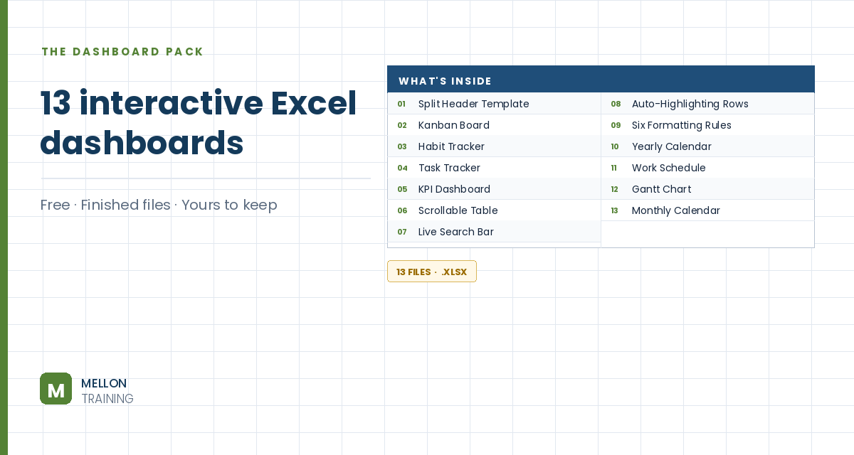
What’s in the pack
Free, instant, and yours to keep.
No spam, ever. Unsubscribe with one click.
One practical Excel tip a week.
Watch the 15-minute video or follow the written steps below. The finished tracker is in the free pack above.
A daily task tracker with drop-downs for priority and status, colour-coded priorities, live counts at the top and a progress bar that fills as you complete tasks. No macros and only one formula.
Select the whole sheet. Set the row height to 20, the column width to 15 and the font size to 14, and align text middle-left.
In B7:F7 type the headers No., Task, Priority, Status and Notes. Select B7:F17, go to Insert > Table and tick My table has headers. Tables grow automatically and carry their formatting and formulas with them. Turn off gridlines from the View tab.
On Table Design, choose New Table Style: give the whole table a light grey outline and inside borders, and the header row bold text with a very light grey fill. Apply it. Then type Tasks in the Table Name box. Add a few example tasks.
Click just above the Priority header to select the column, then go to Data > Data Validation. Set Allow to List and type the source as High,Medium,Low.
With the column still selected, go to Conditional Formatting > New Rule > Format only cells that contain, set equal to High and pick a light red fill. Repeat for Medium (light blue) and Low (light green).
Type Not started, In progress and Completed in B2, C2 and D2. Select the Status column, open Data Validation, choose List and point the source at B2:D2. If you later rename a status, the drop-down picks it up.
Fill B2:B5, C2:C5 and D2:D5 with light red, blue and green, and merge B3:B5, C3:C5 and D3:D5. In B3:
=COUNTIF(Tasks[Status],B2)
It counts how many tasks in the table’s Status column match the word in B2. Copy it to C3 and D3, changing B2 to C2 and D2. Make the results bigger and change a few statuses to watch them update.
Select B2:D5 and insert a 100% Stacked Bar chart. In Select Data, click Switch Row/Column so the three statuses form one bar, order them Not started, In progress, Completed, and untick the extra axis labels. Set the gap width to 0, colour the pieces red, light blue and light green, then delete the title, axes and legend and remove the chart fill and border.
In the first No. cell (B8) enter =ROW()-7. The table copies it down, so new rows number themselves. Drag the table’s bottom-right handle to add more rows: drop-downs and colours come along. To track another project, copy the sheet with Move or Copy > Create a copy.
YOUR NEXT STEP
Every dashboard in this pack rests on the same three techniques: conditional formatting, data validation and dynamic formulas. Learn those properly and you stop collecting templates — you build whatever the job actually needs.
30-day money-back guarantee, handled by Udemy. No forms, no questions.
★★★★★ Join 80,000+ students
Andreas Exadaktylos · Microsoft-certified Excel instructor · mellontraining.com
WATCHING ON YOUTUBE?
11 step-by-step courses on Excel, Power BI, Python and AI, all on Udemy with lifetime access.