
THE MACRO PACK
Import them once and they work in every workbook you open — plus three macro-enabled files from my VBA videos. Free, instant, yours to keep.
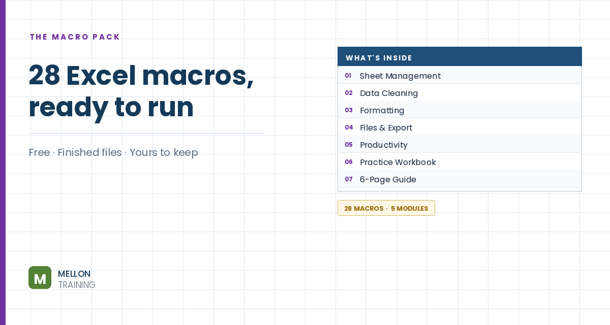
What’s in the pack
Free, instant, and yours to keep.
No spam, ever. Unsubscribe with one click.
One practical Excel tip a week.
Watch the 13-minute video or follow the written steps below. The macro pack above includes the finished workbook with the full code.
Instead of three worksheets, you keep three tables side by side on one sheet and use clickable tab shapes to show one at a time. The example sheet is called Region Tabs, with North data in columns B:G, Central in I:N and South in P:U, and space above them for the tabs.
Go to Insert > Shapes and choose a Rounded Rectangle. Draw it above the tables, then on the Shape Format tab set it to about 0.5″ high and 1.5″ wide. Give it a strong fill colour (this is the active look), set Shape Outline to No Outline, and type North. Make the text bold, slightly bigger and centred both ways.
Hold Ctrl and drag the shape to the right to copy it (add Shift to keep it level). Do it again, so you have three tabs, and change their text to Central and South.
Select all three tabs and Ctrl+drag them to make copies. Give the copies a lighter style, such as pale grey, so they clearly look inactive. You now have six shapes.
The code finds shapes by name, so this matters. Click a shape, click in the Name Box left of the formula bar, type the new name and press Enter (if you don’t press Enter, the name isn’t saved). Use North_On, North_Off, Central_On, Central_Off, South_On and South_Off, with underscores rather than spaces. You can check them all in Page Layout > Selection Pane.
Select North_On and North_Off together, then use Shape Format > Align > Align Left and then Align Top. Repeat for Central and South. You’ll now see just one set of tabs.
Turn on the Developer tab if you need to (right-click the ribbon > Customize the Ribbon > tick Developer). Open Developer > Visual Basic (or press Alt+F11) and choose Insert > Module. You need one macro per tab, TabNorth, TabCentral and TabSouth. Each one hides the other regions’ columns, shows its own, and shows its own “on” shape while showing the “off” shapes for the others. For example:
Sub TabNorth()
    Columns("H:U").Hidden = True
    Columns("B:G").Hidden = False
    With ActiveSheet.Shapes
        .Item("North_On").Visible = True
        .Item("North_Off").Visible = False
        .Item("Central_On").Visible = False
        .Item("Central_Off").Visible = True
        .Item("South_On").Visible = False
        .Item("South_Off").Visible = True
    End With
End Sub
TabCentral and TabSouth follow the same pattern with their own columns and shapes. Make sure the column letters match where your tables are, and the shape names match exactly. Save the file as an Excel Macro-Enabled Workbook (.xlsm), or the macros won’t be kept.
In the Selection Pane, select both North shapes, right-click the North tab, choose Assign Macro and pick TabNorth. Do the same for Central and South.
Select all the tab shapes, right-click and choose Size and Properties, then under Properties choose Don’t move or size with cells. Now inserting rows or columns won’t push them around.
Click each tab: only that region’s table should show, with its tab highlighted. If nothing happens, check that macros are enabled, the column letters in the code match your tables, the shape names are spelled exactly the same as in the Selection Pane, and each tab has the right macro assigned. It’s usually a small spelling mismatch.
YOUR NEXT STEP
Recording a macro is where everyone starts, and it gets you a long way. The moment you need it to do something slightly different, you have to read what Excel wrote and change it. Open any module in this pack — the comments show you what every line does. That’s the whole leap, and it’s smaller than people expect.
30-day money-back guarantee, handled by Udemy. No forms, no questions.
★★★★★ Join 80,000+ students
Andreas Exadaktylos · Microsoft-certified Excel instructor · mellontraining.com
WATCHING ON YOUTUBE?
11 step-by-step courses on Excel, Power BI, Python and AI, all on Udemy with lifetime access.