
THE CHART PACK
The finished chart from the video with the helper columns left visible — plus 21 more advanced charts. Free, instant, yours to keep.
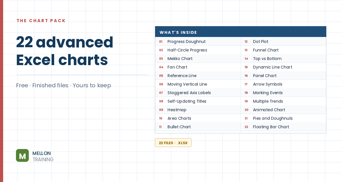
What’s in the pack
Free, instant, and yours to keep.
No spam, ever. Unsubscribe with one click.
One practical Excel tip a week.
Watch the 10-minute video or follow the written steps below. The finished chart is in the free pack above.
When a column chart has negative values, the bars run into the axis labels. This trick staggers the labels: years with profits get their label below the axis, years with losses get it above, and it updates by itself. The example shows ten years of profit for a tech company, with losses in 2019 to 2021.
Select the table (B2:C12), go to Insert > Recommended Charts and choose Clustered Column. The three negative bars cover the year labels. (Setting the axis Label Position to Low moves all labels to the bottom, but staggering them keeps each label next to its bar.)
Right-click a bar, choose Format Data Series > Fill & Line > Solid fill and tick Invert if negative. Pick green for positive values and red for negative ones.
These act as invisible rails along the zero line, one for each set of labels. Name them +labels and -labels (type an apostrophe first, ‘+labels, or Excel treats the plus sign as a formula). In D3:
=IF(C3>=0,0,NA())
In E3:
=IF(C3<0,0,NA())
Each shows 0 only for its own kind of year. NA() returns #N/A, which a chart simply skips. Copy both down.
Copy the two helper columns with their headers, click the chart and paste. Go to Chart Design > Change Chart Type > Combo and set both helper series to Line. Two flat lines appear along the zero axis.
Right-click the +labels line, choose Add Data Labels, then Format Data Labels. Set the position to Below, tick Value From Cells and select the years (B3 down). Untick Value and Show Leader Lines. Under Text Box, set all margins to 0 and untick Wrap text in shape. Do the same for the -labels line, but set the position to Above.
Format the horizontal axis: set Label Position to None and give the axis a solid black line about 1.5 pt wide. Set both helper lines to No line: the labels stay, the lines vanish.
Delete the gridlines and vertical axis and remove the chart border. Add data labels to the bars, a title, and any notes you need, and set the gap width to about 50%. Change a value from positive to negative and the bar colour and label position switch automatically.
YOUR NEXT STEP
NA() returns #N/A, and an Excel chart skips #N/A entirely rather than plotting it as zero. That one behaviour is what lets you split data across two series and position labels independently. The fan chart and the panel chart in this pack use the same idea — once you know it, you stop needing a tutorial per chart.
30-day money-back guarantee, handled by Udemy. No forms, no questions.
★★★★★ Join 80,000+ students
Andreas Exadaktylos · Microsoft-certified Excel instructor · mellontraining.com
WATCHING ON YOUTUBE?
11 step-by-step courses on Excel, Power BI, Python and AI, all on Udemy with lifetime access.