
THE DASHBOARD PACK
Kanban board, habit tracker, KPI report, search bar and more — built, working, ready to take apart. Free, instant, yours to keep.
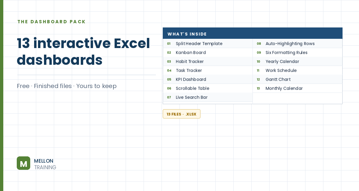
What’s in the pack
Free, instant, and yours to keep.
No spam, ever. Unsubscribe with one click.
One practical Excel tip a week.
Watch the 11-minute video or follow the written steps below. The finished scrollable table is in the free pack above.
When you scroll down a long table, any charts beside it scroll away too. The fix: show a fixed “window” of rows that changes as you move a scroll bar, so the table updates in place while the charts stay put. The example table has 350 orders on a sheet called Dashboard.
Add a new sheet (the example calls it Dashboard New). Click where the table should start, type = and click the first header on the original table, then drag across to bring in the rest of the headers.
If you don’t see the Developer tab, go to File > Options > Customize Ribbon and tick Developer. Then go to Developer > Insert and choose the Scroll Bar under Form Controls (not ActiveX). Draw it to the right of where the table will be.
Its arrows can look very faint, but it still works. If you want obvious arrows, a Spin Button from Form Controls does the same job.
Right-click the scroll bar, choose Format Control, and set Cell link to an out-of-the-way helper cell such as N3. Set the Minimum value to 1 and, for now, the Maximum value to 350. Move the scroll bar and check that N3 changes.
In the first data cell under your headers (A2), enter:
=OFFSET(Dashboard!A2,$N$3,0)
OFFSET starts at the first data cell of the original table, moves down by the number in N3, and doesn’t move across (0). Press F4 on the N3 reference to lock it with dollar signs before copying. Copy the formula across the row for the other columns, then down for as many rows as you want visible at once (15 or 20, for example). Format the amount column as currency and the date column as a date.
If you scroll all the way down and see zeros or blanks, the maximum is too high: whatever value the scroll bar is on becomes the top row of the window, so at 350 there’s nothing left to show below it. Set the maximum so the last record lands on the bottom row instead: total rows minus visible rows. With 350 rows and 14 visible, that’s 336. Or scroll until the last record sits at the bottom and read the number in N3.
Copy your charts onto the new sheet and position them beside the table. Turn off gridlines and format the headers. Now the table scrolls and the charts stay exactly where they are.
YOUR NEXT STEP
Every dashboard in this pack rests on the same three techniques: conditional formatting, data validation and dynamic formulas. Learn those properly and you stop collecting templates — you build whatever the job actually needs.
30-day money-back guarantee, handled by Udemy. No forms, no questions.
★★★★★ Join 80,000+ students
Andreas Exadaktylos · Microsoft-certified Excel instructor · mellontraining.com
WATCHING ON YOUTUBE?
11 step-by-step courses on Excel, Power BI, Python and AI, all on Udemy with lifetime access.