How to Create a Pareto Chart in Excel (80/20 Rule)

Roughly 80% of your problems come from about 20% of the causes. A Pareto chart
is how you find out which 20%.

It combines a column chart with a cumulative percentage line, so the few items
driving most of the total become obvious at a glance. In this tutorial we build
one from scratch — sorting the data, adding the cumulative column, and getting
the secondary axis to line up properly.

Watch: a Pareto chart in 4 minutes

Prefer reading? The same steps are written out below the video.

Step-by-step

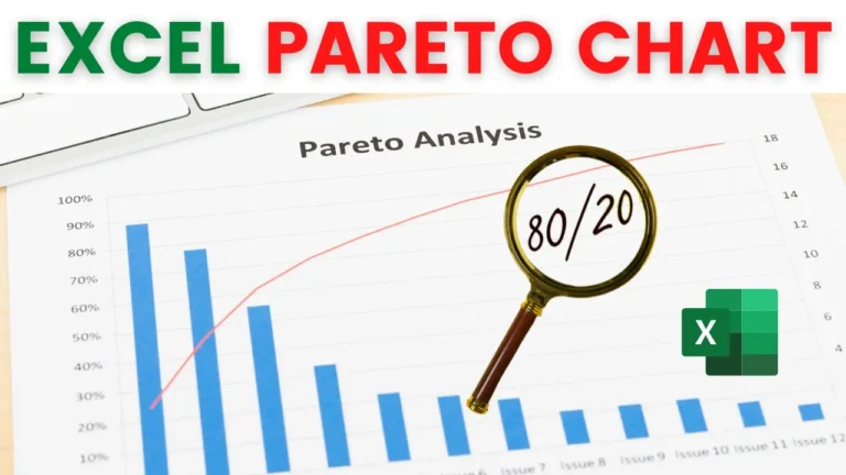
The example uses two columns: item category and sales. The finished chart shows sales as columns and the cumulative percentage as a line.

1. Sort sales from largest to smallest

This matters: a Pareto chart only works when the values are in descending order. Click any value in the sales column, then go to Home > Sort & Filter > Sort Largest to Smallest.

2. Add a total

Click the cell under the last sales value (B9 in the example), click AutoSum and press Enter.

3. Add a cumulative column

Type Cumulative as the header in column C. The first entry is just the first sales value, so in C2 type =B2. Every row after that adds the previous cumulative total to the current sales value, so in C3 type =C2+B3. Then double-click the fill handle to copy it down.

4. Add a percent column

Type Percent as the header in column D. In D2, divide the cumulative value by the total: =C2/$B$9. Press F4 after clicking B9 to make it an absolute reference, so it stays fixed as you copy the formula down. Fill it down, then click Percent Style on the Home tab.

5. Insert the chart

Select the category, sales and percent columns, but not the cumulative column (hold Ctrl to select columns that aren’t next to each other). Go to Insert > Recommended Charts. The first suggestion, Clustered Column – Line on Secondary Axis, is exactly what you need. Click OK.

6. Label the line

Click the line, then go to Chart Design > Add Chart Element > Data Labels > Below, so each point shows its exact percentage.

Reading the result

In the example, the first three categories (refreshments, spirits and mineral water) make up almost 80% of total sales. That’s the “vital few” a Pareto chart is designed to reveal.

Go further

My course Excel Charts, Infographics & Data Visualisation walks through 50+ advanced, dynamic charts in 90 lessons.