
THE CHART PACK
Mekko, fan chart, bullet, gauge, waterfall — the ones Excel won’t build for you. All finished and working. Free, instant, yours to keep.
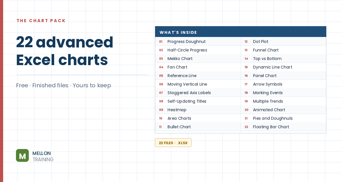
What’s in the pack
Free, instant, and yours to keep.
No spam, ever. Unsubscribe with one click.
One practical Excel tip a week.
Watch the 9-minute video or follow the written steps below.
A milestone chart plots key dates on a timeline, so you can see both the milestones and the gaps between them. It’s ideal for planning a project or reporting check-ins and deliverables.
The example has dates in B3:B10 and activities in C3:C10. Add three helper columns:
=IF(B3<>"",B3,"") shows the date only if there is one.=IF(AND(C3<>"",E3<>""),C3,"") shows the activity only if it has both a date and a name.=IF(F3<>"",10,"") sets how high the label sits. Any number works.Copy all three down to row 10.
Click an empty cell and go to Insert > Line with Markers. You’ll get a blank chart area.
Go to Chart Design > Select Data > Add. Name the series Date and select F3:F10 as its values. Excel draws a flat line along zero. Then click Edit under Horizontal (Category) Axis Labels and select the dates in column E, so the axis shows dates.
Add a second series named Activity with G3:G10 as its values, then click OK.
Right-click one of the activity points, choose Change Series Chart Type, and in Combo set the Activity series to Stacked Column. Then right-click the columns, choose Format Data Series and put them on the Secondary Axis. Delete the new vertical axis on the right.
Go to Select Data, select the Activity series and edit its horizontal axis labels to F3:F10. Then right-click a column, choose Add Data Labels, and in Format Data Labels tick Category Name only, with the label position set to Inside End.
Select the columns and go to Add Chart Element > Error Bars > More Error Bar Options. Choose Minus, No Cap and a Percentage of 100%. Then give the columns No fill and No border, so only the error-bar lines remain, connecting each label to the timeline.
Click the horizontal line, choose Format Data Series and set the line to No line. Under Marker, choose a built-in diamond, size 10, in green. Finish with a title, axis font changes, or label tweaks as you like.
YOUR NEXT STEP
Almost every “how did they build that” chart is the same idea — a helper column feeding an invisible series. Once you spot the pattern you stop needing tutorials. You look at a chart and think “that’s two series stacked, one of them hidden”, and you’re usually right.
30-day money-back guarantee, handled by Udemy. No forms, no questions.
★★★★★ Join 80,000+ students
Andreas Exadaktylos · Microsoft-certified Excel instructor · mellontraining.com
WATCHING ON YOUTUBE?
11 step-by-step courses on Excel, Power BI, Python and AI, all on Udemy with lifetime access.