How to Use Data Bars, Icon Sets and Symbols in Excel

Step-by-step

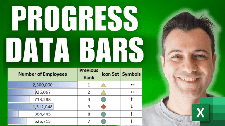
When a dashboard has no room for a chart, data bars, icon sets and symbols show trends inside the cells. The example is a table of 50 companies with their country, employees, and their rank this year (column A) and last year (column E).

1. Add data bars

Select the employee numbers (D2:D51) and go to Home > Conditional Formatting > Data Bars and pick a gradient fill. Each cell gets a mini bar sized against the smallest and largest values in the range. Use Manage Rules > Edit Rule to set the minimum, maximum or bar style yourself.

2. Work out whether each rank went up or down

In F2, return 0 for no change, -1 if the rank got worse (a higher number) and 1 if it improved:

=IF(A2=E2,0,IF(A2>E2,-1,1))

Copy it down to F51.

3. Turn the results into icons

Select F2:F51 and go to Conditional Formatting > New Rule > Format all cells based on their values. Set Format Style to Icon Sets and choose a three-icon set. Change the types to Number: green when the value is > 0, yellow when >= 0 (which now only catches zero), and red for the rest. Tick Show Icon Only. Icons read well even when the dashboard is printed in black and white.

4. Use arrow symbols from a font

Another option is special characters. In the Wingdings 3 font, # shows as an up arrow, $ as a down arrow and 1 as a double-headed arrow (check them via Insert > Symbol). In G2:

=IF(F2=1,"#",IF(F2=-1,"$","1"))

Copy it down, then set column G to the Wingdings 3 font and make it bold. The characters turn into arrows.

5. Put it together

Bars, icons and arrows give an at-a-glance view of what’s up, down or flat, in a fraction of the space a chart would take. The same technique works in PivotTables and formulas too.

Go further

My Excel Dashboard & Data Analysis Masterclass course shows how to build these into complete dashboards.