
THE CHART PACK
The finished chart from the video, MINIFS and MAXIFS helper columns included. Plus 21 more advanced charts, free.
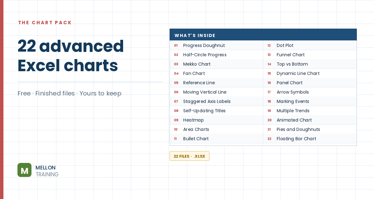
What’s in the pack
Free, instant, and yours to keep.
No spam, ever. Unsubscribe with one click.
One practical Excel tip a week.
Watch the 8-minute video or follow the written steps below. The finished chart is in the free pack above.
A floating bar chart shows a low-to-high range for each item, with bars that start at the low value instead of zero. The example compares each salesperson’s lowest and highest sale. Excel has no floating bar chart type, but a line chart with up/down bars does the job.
The data has sale values in C3:C12 and salesperson names in D3:D12. Put the names across a header row (H2:L2). In H3, find the lowest sale for the name above:
=MINIFS($C$3:$C$12,$D$3:$D$12,H$2)
In H4, the highest:
=MAXIFS($C$3:$C$12,$D$3:$D$12,H$2)
Copy both across to column L. The dollar signs keep the ranges fixed when you copy. If the results look wrong, check those first.
Select H2:L4, go to Insert > Line and choose the first 2-D line chart. Move and resize it.
Click the + (Chart Elements) button and tick Up/Down Bars. Excel draws a bar between the low and high line for each person: those are your floating bars.
Right-click a bar and choose Format Up Bars. In the video the bars get a Gradient fill (Linear Down) with green at the top and red at the bottom, plus a thin blue border. Any fill works: the gradient just shows what’s possible.
Right-click the first line, choose Format Data Series > Fill & Line > No line. Repeat for the second line. Only the floating bars remain.
Delete the legend, add a title such as Sales comparison, and remove the chart border (Format > Shape Outline > No Outline). At a glance you can now compare each person’s lowest and highest sale.
YOUR NEXT STEP
That’s the whole floating bar: a stacked chart where the first segment is switched off. The waterfall chart works the same way. So does the Gantt. Once you know Excel’s advanced charts are mostly ordinary charts with parts hidden, you stop needing a tutorial for each one — you can see how they’re built.
30-day money-back guarantee, handled by Udemy. No forms, no questions.
★★★★★ Join 80,000+ students
Andreas Exadaktylos · Microsoft-certified Excel instructor · mellontraining.com
WATCHING ON YOUTUBE?
11 step-by-step courses on Excel, Power BI, Python and AI, all on Udemy with lifetime access.