
THE DASHBOARD PACK
10 Excel dashboards, finished and free
Kanban board, habit tracker, KPI report, search bar and more — built, working, ready to take apart. Free, instant, yours to keep.
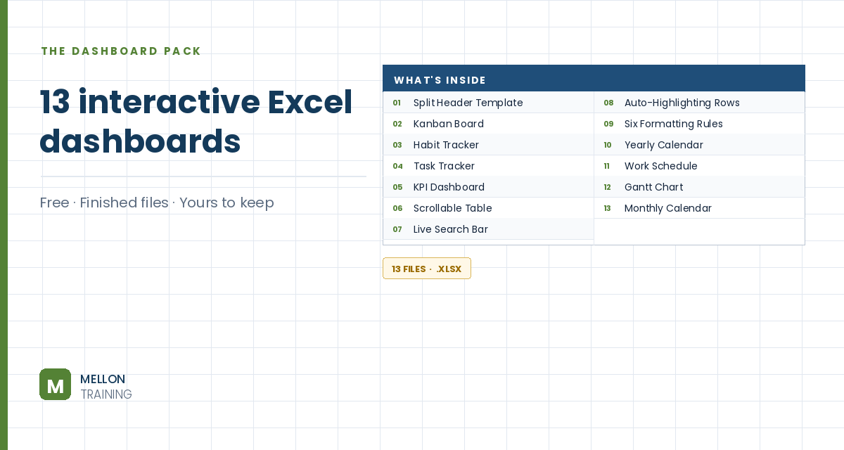
What’s in the pack
- Kanban board, habit tracker and task tracker, all working
- A full KPI dashboard with SUMIFS, COUNTIFS and slicers
- Live search bar and scrollable table — no VBA in either
- The split-header template, three ways
- Works in Excel 365, 2021 and 2019 — PC and Mac
Send it to my inbox
Free, instant, and yours to keep.
No spam, ever. Unsubscribe with one click.
One practical Excel tip a week.
How to Make an Excel Dashboard Step by Step
Watch the 12-minute video or follow the main stages below. The free dashboard pack above has ten more finished dashboards to learn from.
The build, stage by stage
You’ll turn an order sales table (order date, customer, region, item, units and total) into a one-page dashboard: key metrics, a top-3 customers table, a quarterly trend line, a doughnut chart by region, a column chart of best-selling items, and slicers to filter it all.
1. Decide what to track first
Before designing anything, ask: what problem am I trying to solve? Pick the metrics, or KPIs, that answer it. Everything on the dashboard should support those.
2. Create the metrics
Click in the data and go to Insert > PivotTable, placing it on a new sheet you rename Dashboard. Drag Total into Values, then Units. Right-click a value, choose Number Format, and set no decimals with a thousands separator. To try other calculations (count, average, max, min), right-click and use Summarize Values By.
3. Add a top-3 customers table
Insert another PivotTable from the same data, this time on the existing Dashboard sheet (cell A9 in the example). Put Customer in Rows and Total in Values. Use the row filter: Value Filters > Top 10, changed to 3. Then right-click and choose Sort Largest to Smallest.
4. Build the quarterly trend line
Create a PivotTable on a new sheet (Year-Quarter) with Order Date in Rows and Total in Values. Right-click a date, choose Group and select Quarters and Years. Then insert a PivotChart as a line chart and keep it simple: delete the legend and title, hide the field buttons (Field Buttons > Hide All) and remove the gridlines. Use Move Chart to place it on the Dashboard sheet.
5. Add the doughnut, column chart and slicers
Follow the same pattern for the remaining pieces: a PivotTable and doughnut chart showing each region’s share of the total, and a column chart of the items with the most units, both moved onto the Dashboard. Finally, add slicers so you can filter the whole dashboard with a click.
6. Finish the layout
On the View tab, untick Gridlines, Formula Bar and Headings, so the dashboard looks like a clean report rather than a spreadsheet.
YOUR NEXT STEP
You've got ten. The course builds ten more, from scratch.
Every dashboard in this pack rests on the same three techniques: conditional formatting, data validation and dynamic formulas. Learn those properly and you stop collecting templates — you build whatever the job actually needs.
- Ten complete dashboards, blank file to finished
- Slicers, timelines, dynamic charts and KPI cards
- Every workbook and dataset included
- 180 lessons, 21 hours · lifetime access · all future updates
30-day money-back guarantee, handled by Udemy. No forms, no questions.
★★★★★ Join 80,000+ students
Andreas Exadaktylos · Microsoft-certified Excel instructor · mellontraining.com
No matter your profession, stop wasting precious hours crunching numbers.
Get the Excel training that builds an unbeatable resume and warp drives your career.