How to Create a Dynamic Calendar in Excel (Holidays and Today Highlighted)

Build a calendar in Excel that rebuilds itself. Pick a month and year from two
dropdowns and the whole grid redraws — dates in the right weekday columns,
today highlighted automatically, and your public holidays marked in their own
colour.

Step by step, from a blank sheet. You’ll have a calendar you actually reuse.

Watch the full build

Prefer reading? The main steps and formulas are written out below the video.

Step-by-step

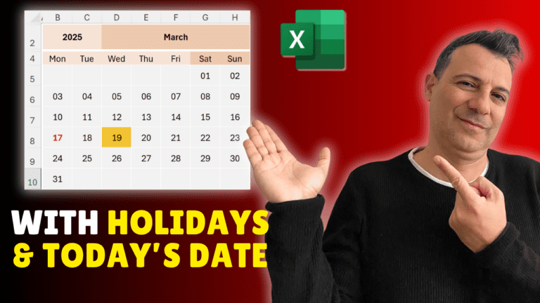
You’ll build a calendar that redraws itself when you pick a different month or year from two drop-downs, with today’s date and your holidays highlighted automatically. It uses SEQUENCE, so you need Excel 365 or Excel 2021.

1. Add year and month drop-downs

On a helper sheet (the example calls it Year Month List), list the years 2000 to 2030 in one column and the 12 month names in another. On the calendar sheet, click B2, go to Data > Data Validation > List and select the years as the source. Do the same in D2 with the months.

2. Lay out the grid

Type Monday to Sunday across B4:H4. Set columns B:H to a width of about 5 and centre them. The dates go in a 6-row by 7-column grid (B5:H10), because a month can span six weeks; set those rows to about 30 high. Add colour to taste: the video uses light orange for weekdays, a darker orange for weekends, a light grey fill and thick white borders for the date cells, with gridlines turned off.

3. Find the first day of the month

In K5 type First date, and in L5:

=DATEVALUE(1&D2&B2)

This joins 1, the month name and the year into text Excel can read as a date. Format L5 as a date.

4. Find which weekday it falls on

In K6 type Start day, and in L6:

=WEEKDAY(L5,2)

The 2 makes Monday = 1 through Sunday = 7, which matches the grid.

5. Fill the grid with real dates

In B5:

=SEQUENCE(6,7,L5-L6+1,1)

SEQUENCE fills 6 rows by 7 columns, counting up by 1. Starting at L5-L6+1 shifts the first number back so the 1st of the month lands under the right weekday. Select B5:H10, open Format Cells > Custom and type dd so the cells show day numbers.

6. Highlight today

Select B5:H10, go to Conditional Formatting > New Rule > Use a formula, enter =B5=TODAY() and choose an orange fill.

7. Hide dates from other months

To show only the selected month, replace the formula in B5 with one that keeps a date only if its month matches L5 and shows a blank otherwise, for example:

=IF(MONTH(SEQUENCE(6,7,L5-L6+1,1))=MONTH(L5),SEQUENCE(6,7,L5-L6+1,1),"")

8. Mark holidays automatically

Add a sheet called Holidays and list your holiday dates in B2:B20. Back on the calendar, select B5:H10 and add another conditional formatting rule with the formula:

=COUNTIF(Holidays!$B$2:$B$20,B5)>0

Format it as bold red text. Any holiday on your list now stands out whenever its month is shown.

Try it

Pick a different month or year and the whole calendar updates instantly. From here you can add colour-coded events, or expand it into a yearly or weekly planner.

Go further

My Excel Tips & Shortcuts: 100+ Powerful Hacks course collects a hundred small techniques like these that add up to hours saved every week.