
Prefer reading? The main stages are written out below the video.
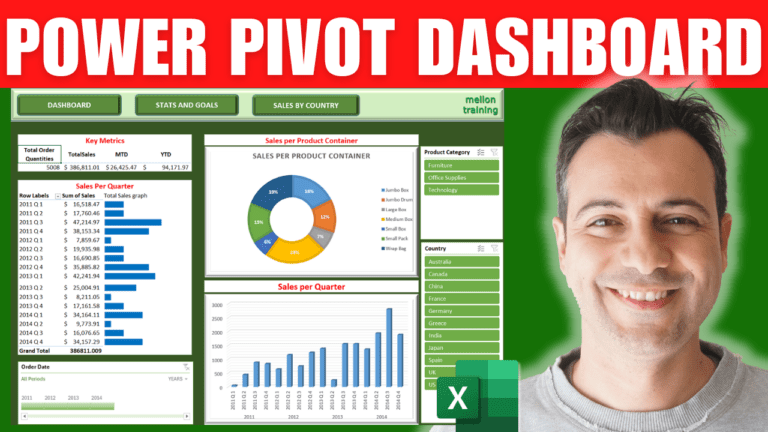
A complete interactive dashboard over three sheets, built on data already loaded into the Power Pivot data model with measures for total quantities, month-to-date and year-to-date sales. No add-ins, no VBA.
Draw a rectangle across the top (A1:Q4), give it a light green gradient fill and a bevel effect. Add three rounded rectangles as buttons with a convex bevel, select them with Shift, and use Align Middle and Distribute Horizontally. Label them Dashboard, Stats and Goals and Sales by Country (bold, size 14, centred). Add your logo top right, narrow column A and turn off gridlines.
Use Move or Copy > Create a copy to make the other two sheets with the same header, and rename all three. Right-click each button > Link > Place in This Document and point it at the matching sheet.
Click B8, open Power Pivot > Manage > PivotTable into the existing sheet, and tick the three measures: total order quantity, sales month-to-date and year-to-date. Add a red Key metrics title above, and format the values as currency.
Add a second PivotTable at B12 with Quarter in Rows and Sales in Values. Next to it, draw bars with REPT:
=REPT("g",C13/5000)
REPT repeats the letter g once for every 5,000 in sales. Fill down, set the font to Webdings (g becomes a square) and colour it blue. Use a bigger divisor if the bars get too long.
From Power Pivot, insert a PivotChart at G8 with Product Container on the axis and Sales as values; change it to a Doughnut, apply chart style 8 for percentage labels, and hide the field buttons. Insert another at G23 with year and quarter on the axis and a count of Order ID, as a 3-D Clustered Column.
Go to Insert > Timeline, choose Data Model > This Workbook Data Model and tick Order Date. Then Insert > Slicer the same way for Country and Product Category. For each one, open Report Connections and tick every PivotTable and chart so one click filters the whole dashboard.
On the second sheet, use Power Pivot > PivotTable > Four Charts at B6 and fill them: a 3-D bar of sales by customer, a 3-D pie of sales by customer segment, a doughnut of sales by product category, and a 3-D column of average sales per year (change the value field setting to Average). Hide field buttons, delete legends you don’t need and give each a clear title.
My Excel Dashboard & Data Analysis Masterclass course builds ten dashboards like this one, every workbook included.