
Prefer reading? The same steps are written out below the video.
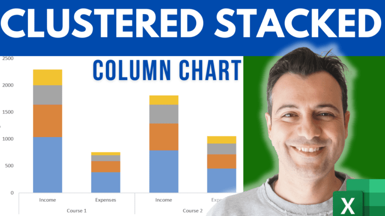
This is the step that makes the chart work. The example has two courses. Each has an Income row and an Expenses row, broken down into four categories: E-learning, YouTube, Webinars and Podcast.
| E-learning | YouTube | Webinars | Podcast | ||
|---|---|---|---|---|---|
| Course 1 | Income | … | … | … | … |
| Expenses | … | … | … | … | |
| Course 2 | Income | … | … | … | … |
| Expenses | … | … | … | … |
Select the whole range (A2:F6 in the example), go to Insert, click the Column Chart button and choose Stacked Column. It won’t look right yet. That’s expected.
Click the chart, open the Chart Design tab (called Design in older versions of Excel) and click Switch Row/Column. Excel now groups the columns by course: an Income column and an Expenses column for each course, each stacked by category.
To check the result, select C3:F3 (the income of Course 1) and look at the Sum in the status bar. It matches the height of Course 1’s Income column.
Right-click any of the series, choose Format Data Series and set Gap Width to 100%.
Give the chart a title and move the legend to the right.
For a horizontal version, go to Chart Design > Change Chart Type and pick Stacked Bar.
My course Excel Charts, Infographics & Data Visualisation walks through 50+ advanced, dynamic charts in 90 lessons.
WATCHING ON YOUTUBE?
11 step-by-step courses on Excel, Power BI, Python and AI, all on Udemy with lifetime access.