
THE CHART PACK
Mekko, fan chart, bullet, gauge, waterfall — the ones Excel won’t build for you. All finished and working. Free, instant, yours to keep.
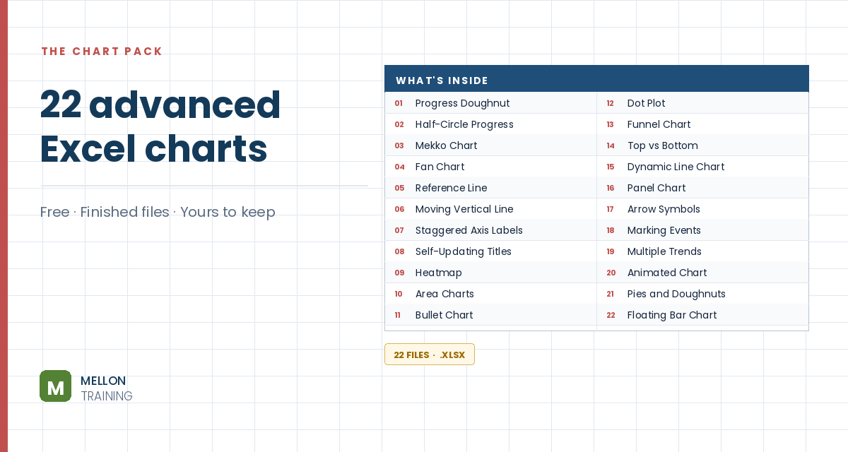
What’s in the pack
Free, instant, and yours to keep.
No spam, ever. Unsubscribe with one click.
One practical Excel tip a week.
Watch the 6-minute video or follow the written steps below. The free chart pack above has 20 more advanced charts, finished and working.
A burndown chart plots the work left to do against time, so you can see at a glance whether a task is ahead of or behind schedule, and predict when it will be finished. Remaining work goes on the vertical axis and days along the horizontal.
You need two pieces of data for each day: the planned hours and the actual hours worked. The example task runs 15 days (starting from day 0), with 8 planned hours a day, so 120 planned hours in total. It assumes the actual total is also 120.
Add three calculation columns: Remaining planned, Remaining actual and Done today.
=IF(D6="",NA(),previous remaining − D6). A #N/A keeps the line from dropping to zero on days you haven’t worked yet.Select the Remaining planned and Remaining actual columns and go to Insert > Line Chart. Use the Day column for the horizontal axis labels.
Reading it: the planned line is a straight diagonal (8 hours a day). Where the actual line sits above it, the project is behind schedule, with more work left than planned. Where it sits below, you’re ahead.
Right-click the chart, choose Select Data, click Edit under the horizontal axis labels and select the days including day 0. Delete any extra line you don’t need, and the title.
Right-click the chart, choose Select Data > Add, name the series Done Today, and select its values (G4:G20 in the example). Then right-click the new series, choose Change Series Chart Type and set it to Clustered Column.
Remove the gridlines, adjust the colours and add a legend if you need one. Your burndown chart is ready.
YOUR NEXT STEP
Almost every “how did they build that” chart is the same idea — a helper column feeding an invisible series. Once you spot the pattern you stop needing tutorials. You look at a chart and think “that’s two series stacked, one of them hidden”, and you’re usually right.
30-day money-back guarantee, handled by Udemy. No forms, no questions.
★★★★★ Join 80,000+ students
Andreas Exadaktylos · Microsoft-certified Excel instructor · mellontraining.com
WATCHING ON YOUTUBE?
11 step-by-step courses on Excel, Power BI, Python and AI, all on Udemy with lifetime access.