
THE DASHBOARD PACK
Six conditional formatting rules already built, plus twelve more dashboards that use them properly. Free, instant, yours to keep.
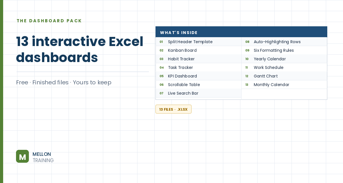
What’s in the pack
Free, instant, and yours to keep.
No spam, ever. Unsubscribe with one click.
One practical Excel tip a week.
Watch the 6-minute video or follow the written steps below. The finished workbook is in the free pack above.
Trend-based conditional formats compare each value with the rest of the range and format it by rank, so trends and outliers jump out. The example uses waste-management data for Australian states.
Select the landfill figures (E29:E36) and go to Home > Conditional Formatting > Color Scales. Hover to preview, then choose Red – Yellow – Green, so high landfill shows red and low shows green.
Colour scales work on blocks of data too, not just one column or row. Select the recovery rates by region (C17:H24) and choose Green – Yellow – Red, so high recovery is green this time.
Colour scales can look busy without a key. To remove one, select the cells and go to Conditional Formatting > Clear Rules > Clear Rules from Selected Cells (or from the entire sheet).
With the same cells selected, go to Conditional Formatting > Data Bars and pick a light blue. Each cell gets a bar like a mini chart: long for big values, short for small ones. Left-align the numbers and make them size 9 so they sit neatly over the bars.
To show icons next to the numbers rather than on them, link a column to the growth rates: in J17 type =I17 and double-click the fill handle to copy it down. Select the new column and go to Conditional Formatting > Icon Sets > 3 Triangles.
By default Excel splits the values into thirds, which isn’t what you want here. Go to Conditional Formatting > Manage Rules (switch the list to This Worksheet to see every rule), select the icon set rule and click Edit Rule. Change both types from Percent to Number. Set green to > 0 and yellow to >= 0. Because positive values already get green, yellow now only catches exactly zero, and everything negative gets red. Tick Show Icon Only and click OK.
Now a green triangle means growth, a red one means a fall, and a yellow line means no change.
YOUR NEXT STEP
Excel’s built-in colour scales tell you which numbers are biggest. What a manager usually wants to know is what changed. That gap — between what the button does and what the report needs — is where formula-based rules come in, and it’s the difference between a coloured spreadsheet and a dashboard.
30-day money-back guarantee, handled by Udemy. No forms, no questions.
★★★★★ Join 80,000+ students
Andreas Exadaktylos · Microsoft-certified Excel instructor · mellontraining.com
WATCHING ON YOUTUBE?
11 step-by-step courses on Excel, Power BI, Python and AI, all on Udemy with lifetime access.