
THE CHART PACK
The finished chart from the video, with the staggered data and divider table left visible. Plus nineteen more advanced charts. Free, yours to keep.
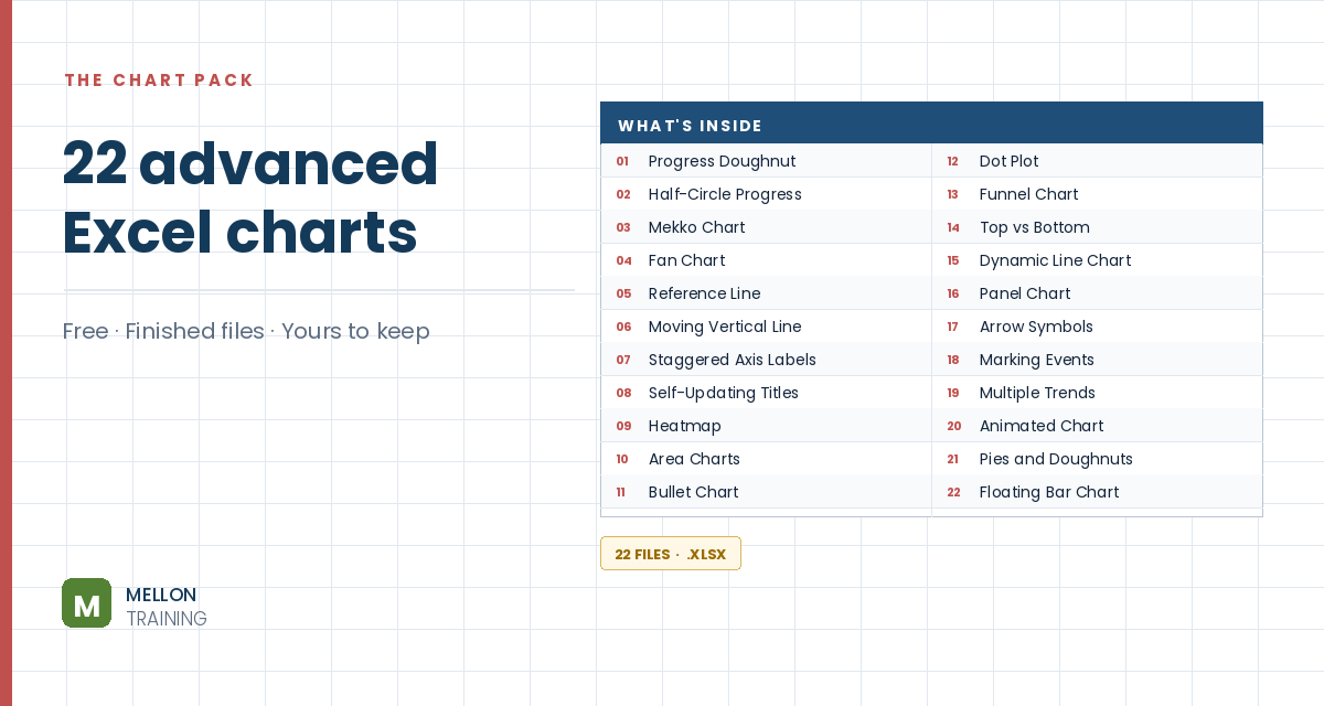
What’s in the pack
Free, instant, and yours to keep.
No spam, ever. Unsubscribe with one click.
One practical Excel tip a week.
Watch the 9-minute video or follow the written steps below. The finished chart is in the free pack above.
A panel chart shows several years side by side in one chart, with a divider between each year and the same colour for each category throughout. The example compares monthly sales of three supermarket categories over four years. A plain line chart of that data is a tangle; a panel chart is easy to read.
Lay the data out so each category has two columns that alternate year by year: one year’s values in the first column, the next year’s in the second, with blanks in between. This staggering is what creates the separate panels.
Select the month column, open Format Cells > Custom and use the type mmmmm. Months show as a single letter (J, F, M…), which saves space on the axis.
Select all the data and insert a 2-D line chart. Move it next to the data and make it bigger. You’ll already see the panel effect, but with six differently coloured series.
Right-click the first series of a category, choose Format Data Series > Fill & Line and set a colour. Give its second series the same colour. In the example: blue for beer, wine and spirits, red for bread and bakery, and green for cleaning products. Delete the title and the duplicate legend entries.
Each year has 12 months, so the dividers sit at 12.5, 24.5 and 36.5. Put 12 in K1. Next to a counter column (1, 2, 3 in J4:J6), enter in K4:
=$K$1*J4+0.5
Copy it down to K6. Put 0 in L4:L6. These are the X and Y positions of the dividers.
Copy K3:L6, select the chart and use Paste Special to add them as a new series (values in columns, categories in the first column). Then go to Change Chart Type > Combo, set the new series to Scatter and tick Secondary Axis. Delete the extra horizontal axis that appears at the top.
Select the scatter series and go to Add Chart Element > Error Bars > More Error Bars Options. Choose direction Plus, end style No Cap, and a fixed value of 1. Then set the right-hand vertical axis maximum to 1 so the lines reach the top.
On that right-hand axis, set tick marks and labels to None. Delete the horizontal error bars, the scatter legend entry and the gridlines. Add a shape style if you like and remove the chart border.
YOUR NEXT STEP
Those panel dividers are error bars on an invisible scatter series. So is the reference line in file 05, and the moving date line in file 06. Three charts that look nothing alike, built the same way. That’s what the course teaches — not fifty recipes, but the handful of patterns underneath them.
30-day money-back guarantee, handled by Udemy. No forms, no questions.
★★★★★ Join 80,000+ students
Andreas Exadaktylos · Microsoft-certified Excel instructor · mellontraining.com
WATCHING ON YOUTUBE?
11 step-by-step courses on Excel, Power BI, Python and AI, all on Udemy with lifetime access.