THE CHART PACK

20 advanced Excel charts, free

Mekko, fan chart, bullet, gauge, waterfall — the ones Excel won’t build for you. All finished and working. Free, instant, yours to keep.

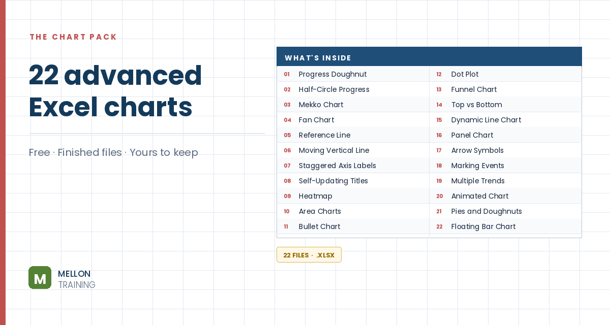
What’s in the pack

20 charts with 37 working chart objects between them
Mekko, fan chart, funnel, bullet, panel and dot plot
Every helper column left visible, so you can see how they work
Self-updating titles, staggered labels, moving date lines
Works in Excel 365, 2021 and 2019 — PC and Mac

Send it to my inbox

Free, instant, and yours to keep.

No spam, ever. Unsubscribe with one click.
One practical Excel tip a week.

How to Create a Bidirectional (Mirror) Bar Chart in Excel

Watch the 3-minute video or follow the written steps below. The free chart pack above has 20 more advanced charts, finished and working.

Step-by-step

A bidirectional (or mirror) bar chart puts two series back to back, with bars running left and right from a central axis. It’s a great way to compare two periods side by side. The example compares sales of three products in 2014 and 2015.

1. Insert a clustered bar chart

Select the data (A1:C4: product names plus the two years) and go to Insert > Clustered Bar.

2. Move the legend to the top

Right-click the legend, choose Format Legend and select Top.

3. Put one series on the secondary axis

Right-click one of the series, choose Format Data Series and select Secondary Axis. The chart now has two horizontal axes, one at the top and one at the bottom.

4. Set matching bounds and reverse one axis

Right-click the secondary axis and choose Format Axis. Set the minimum to the negative of your largest value, the maximum to the positive, and a sensible major unit. The example’s largest value is 5,600, so it uses −6000, 6000 and 1000. Tick Values in reverse order.

Then format the primary axis with the same minimum, maximum and unit, but leave Values in reverse order unticked. The two series now run in opposite directions.

5. Move the product names to the side

The product labels sit in the middle of the chart. Right-click the vertical axis, choose Format Axis, and set Major tick mark and Minor tick mark to None and Label Position to Low.

6. Tidy up

Optionally, hide the minus signs on the axis using a custom number format. Delete the gridlines, add a chart title, and your bidirectional bar chart is ready.

YOUR NEXT STEP

Open any chart. Click Select Data. That's where the trick lives.

Almost every “how did they build that” chart is the same idea — a helper column feeding an invisible series. Once you spot the pattern you stop needing tutorials. You look at a chart and think “that’s two series stacked, one of them hidden”, and you’re usually right.

30-day money-back guarantee, handled by Udemy. No forms, no questions.

★★★★★ Join 80,000+ students

Andreas Exadaktylos · Microsoft-certified Excel instructor · mellontraining.com