
THE DASHBOARD PACK
The finished timeline from the video — it redraws itself when dates change. Plus eleven more Excel files. Free, instant, yours to keep.
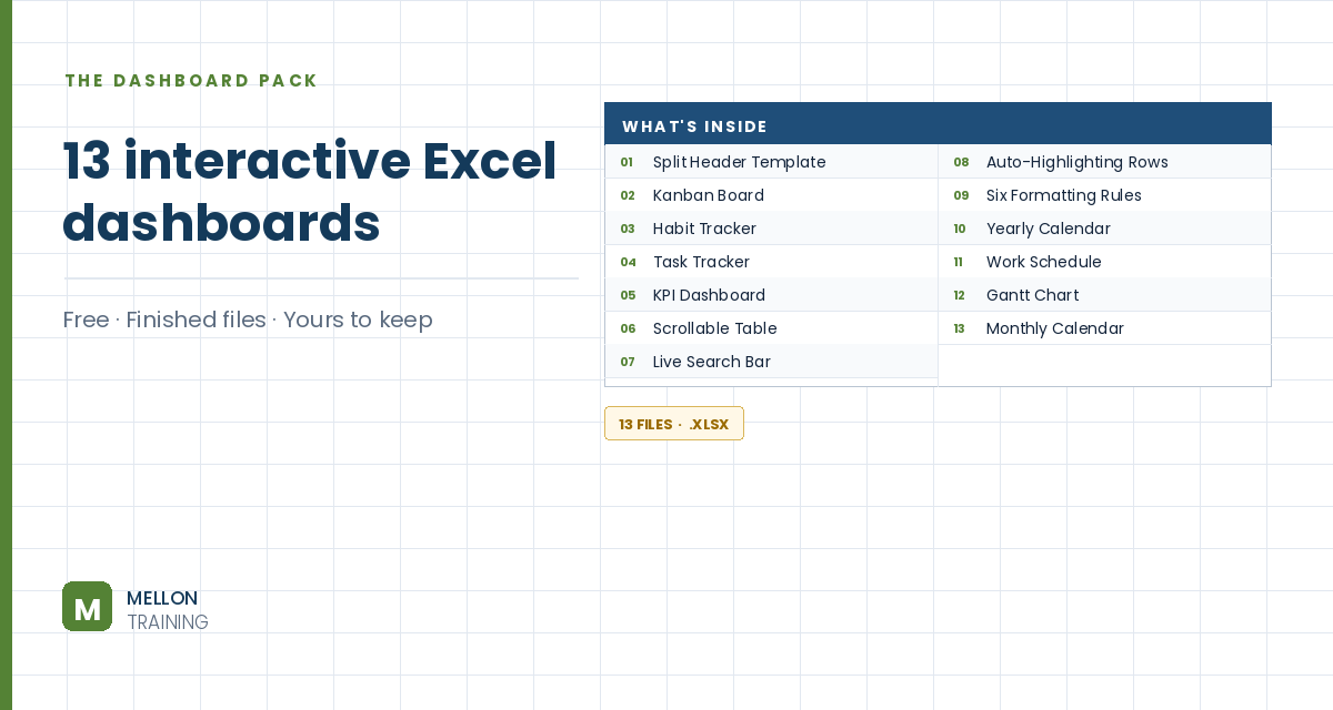
What’s in the pack
Free, instant, and yours to keep.
No spam, ever. Unsubscribe with one click.
One practical Excel tip a week.
Watch the 20-minute build or follow the main stages below. The finished Gantt chart is in the free pack above.
This monthly Gantt chart isn’t a chart object at all. It’s a grid coloured by conditional formatting, so it redraws itself when dates change. It shows years, quarters and months, fills in progress, flags tasks on hold, marks finished tasks and shows where today is.
Add a light grey divider bar across row 4 (out to column AZ). In C2 and C3 add the labels Project start date and Project name, right-aligned. Enter the start date in D2 (the example uses 1 March) with a custom format such as d-mmm-yy, and the project name in D3. Make both bold, white on dark green.
From B4, create eight columns: #, Activity, Assigned to, Start date, End date, Days, Status and % Done. Number the tasks, add some sample activities, format the dates like the project start date, and use size 14 text throughout for a consistent look.
=IF(F5="","",NETWORKDAYS(E5,F5)).To Do,In Progress,On Hold,Done) and a conditional formatting rule that fills “On Hold” light yellow.Turn off gridlines and add thin grey inside and outside borders to the table.
Across the top of the chart area, build three rows: years, then quarters (each merged across three months), then months. Copy the structure across for several quarters, give the month row a light grey fill, and add light grey borders to the whole grid. Use View > Freeze Panes so the task details and timeline headers stay visible as you scroll.
The first month (K3) should be the first day of the quarter that contains your start date, so a June start begins the timeline in April. One way to write it:
=DATE(YEAR($D$2),FLOOR(MONTH($D$2)-1,3)+1,1)
Format it with a custom mmm format (and optionally rotate the text 90°), then fill the next months with =EDATE(K3,1), which moves forward one month at a time. Above it, the year row references the month cell with a yyyy format, and the quarter row converts the month number to Q1–Q4. A conditional formatting rule shades alternate years light grey.
Select the whole grid and add a formula rule that colours a cell when its month falls between the task’s start and end month. Because the timeline uses the first day of each month, compare against first-of-month versions of the dates, for example:
=AND(K$3>=DATE(YEAR($E5),MONTH($E5),1),K$3<=DATE(YEAR($F5),MONTH($F5),1))
Use a light pink fill, and add light borders so the bars read as blocks.
In the grid, a formula returns the letter u only in the month and year that match the task’s end date:
=IF(AND(MONTH(K$3)=MONTH($F5),YEAR(K$3)=YEAR($F5)),"u","")
Paste it across the grid as formulas only, centre and bold it, and change the font to Wingdings, which turns the u into a diamond. Colour it dark pink.
A final rule draws a grey dashed left border on the current month’s column, so you always see where you are: =K$3=DATE(YEAR(TODAY()),MONTH(TODAY()),1).
YOUR NEXT STEP
That Gantt chart isn’t a chart — it’s conditional formatting, data validation and dynamic formulas doing an impression of one. Same three techniques behind the Kanban board and the KPI report sitting next to it in this pack. Learn them properly and you stop looking for templates that almost fit.
30-day money-back guarantee, handled by Udemy. No forms, no questions.
★★★★★ Join 80,000+ students
Andreas Exadaktylos · Microsoft-certified Excel instructor · mellontraining.com
WATCHING ON YOUTUBE?
11 step-by-step courses on Excel, Power BI, Python and AI, all on Udemy with lifetime access.