
THE DASHBOARD PACK
Change one cell — the year — and all twelve months redraw themselves. Plus twelve more Excel files. Free, instant, yours to keep.
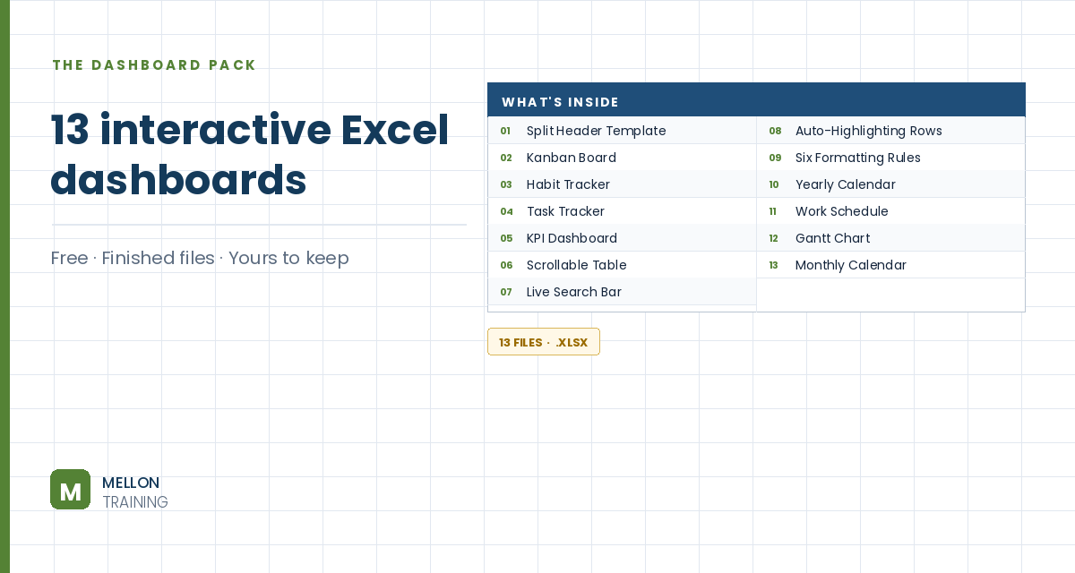
What’s in the pack
Free, instant, and yours to keep.
No spam, ever. Unsubscribe with one click.
One practical Excel tip a week.
Watch the 15-minute video or follow the written steps below. The finished calendar is in the free pack above.
Type a year in one cell and all twelve months redraw themselves. Today’s date is highlighted, days from other months are greyed out, and the whole year prints on one page.
Select the whole sheet. Set the column width to 3.5 and the row height to 25, then centre everything vertically and horizontally. Make columns B:D 18 wide for the helper table, column AC 4 wide and column AD 18 wide. Turn off gridlines from the View tab.
In AD2 type Enter year with white text on dark blue. In AD3 type the year, for example 2026. Make both bold with borders. This one cell drives the whole calendar.
In B2:D2 type the headers Month, 1st and Monday. Fill B3:B14 with 1 to 12. In C3, the first day of each month:
=DATE($AD$3,B3,1)
In D3, the Monday on or before that date, where each month’s grid will start:
=C3-WEEKDAY(C3,2)+1
Fill both down to row 14. For calendars that start on Sunday, use =C3-WEEKDAY(C3,1)+1 instead.
Merge F2:L2 for the month title, with white bold text on dark blue. Give F3:L3 a light blue fill for the weekday labels and type Mo, Tu, We, Th, Fr, Sa, Su. Give the grid F4:L9 all borders, then open Format Cells > Custom and enter d, so each cell shows only the day number.
In F4 enter =$D$3. In G4 enter =F4+1 and copy it across to L4. In F5 enter =L4+1 (the day after the previous row’s Sunday). Copy G4:L4 down to G5:L5, then fill F5:L5 down to row 9. Six rows always cover the whole month.
In the merged title cell F2:
=UPPER(TEXT(L4,"mmmm"))
L4 is always inside the month, so it gives the right name. Make the font white and a little bigger, and give the block light grey inside and outside borders.
Select F4:L9 and go to Conditional Formatting > New Rule > Use a formula:
=MONTH(F4)<>$B$3
Pick a grey font and a light grey fill. Leftover December and February days now fade into the background.
Copy F2:L9 and paste it at N2 for February. In February’s first date cell, change $D$3 to $D$4. In Manage Rules, change the rule’s $B$3 to $B$4. Repeat for each month, moving the references down one row each time.
Select the whole calendar area and add a rule: Format only cells that contain > Cell Value > equal to =TODAY(), with an orange fill. Then hide columns A:D.
Select the calendar range, go to Page Layout > Print Area > Set Print Area, then in File > Print choose Fit Sheet on One Page. Change the year in AD3 any time and everything updates.
YOUR NEXT STEP
A calendar that rebuilds itself from one cell is the same principle as a sales report that rebuilds itself from one dropdown. Date formulas, conditional formatting, dynamic ranges — the same three ideas, pointed at something that matters more. That’s what the course does, ten times over.
30-day money-back guarantee, handled by Udemy. No forms, no questions.
★★★★★ Join 80,000+ students
Andreas Exadaktylos · Microsoft-certified Excel instructor · mellontraining.com
WATCHING ON YOUTUBE?
11 step-by-step courses on Excel, Power BI, Python and AI, all on Udemy with lifetime access.