
THE DASHBOARD PACK
A finished project timeline, built from a stacked bar with one segment hidden. Plus twelve more Excel files. Free, instant, yours to keep.
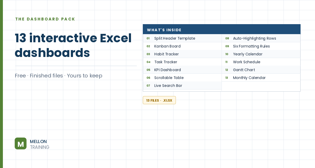
What’s in the pack
Free, instant, and yours to keep.
No spam, ever. Unsubscribe with one click.
One practical Excel tip a week.
Watch the 6-minute video or follow the written steps below. The finished Gantt chart is in the free pack above.
Excel has no Gantt chart type, but a stacked bar chart with one invisible series looks exactly like one. The example plans the stages of building a software application.
List each task on its own row with a Start date and a Duration in working days. The first task, Gather requirements, starts on 8 January and lasts 11 days.
Work out each end date in working days, skipping weekends, with WORKDAY:
=WORKDAY(B3,C3)
Then add a Days in total column that subtracts the start date from the end date, for example =D3-B3, and fill both down.
Hold Ctrl and select three columns: the task names, the start dates and the days in total. Go to Insert > Stacked Bar. It’s not a Gantt chart yet, but it’s close.
Double-click the first (start date) series. In Format Data Series > Fill & Line, choose No fill and No line. The bars still push the visible ones to the right start date, so only the task durations show, floating like a Gantt chart.
Excel stores dates as serial numbers (8 January 2022 is 44569). Double-click the date axis and type the first start date in Minimum and the final end date in Maximum: Excel converts them to serial numbers. Set the major unit to 30 so the gridlines fall roughly once a month.
Set the Gap Width to 0%, colour the bars green and add Data Labels (Center) from Add Chart Element.
Double-click the task axis and tick Categories in reverse order, so the project reads from top to bottom. Delete the title, the legend and the chart border.
YOUR NEXT STEP
A Gantt chart is a stacked bar with the first segment switched off. So is a floating bar, and so is a waterfall. Excel’s advanced charts are mostly ordinary charts with parts hidden — and once you can see that, you stop needing a tutorial for each new one.
30-day money-back guarantee, handled by Udemy. No forms, no questions.
★★★★★ Join 80,000+ students
Andreas Exadaktylos · Microsoft-certified Excel instructor · mellontraining.com
WATCHING ON YOUTUBE?
11 step-by-step courses on Excel, Power BI, Python and AI, all on Udemy with lifetime access.