
THE CHART PACK
The finished heatmap from the video and the raw data behind it — plus 21 more advanced charts. Free, instant, yours to keep.
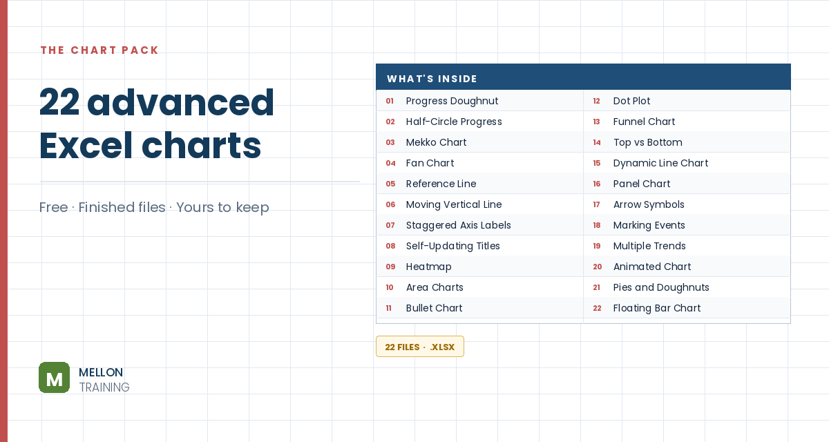
What’s in the pack
Free, instant, and yours to keep.
No spam, ever. Unsubscribe with one click.
One practical Excel tip a week.
Watch the 13-minute video or follow the written steps below. The finished heatmap is in the free pack above.
A heatmap colours each cell by its value, so busy and quiet spots jump out without reading a single number. The example uses five years of coffee shop orders by day of week and hour of day. It’s all conditional formatting and formatting tricks: no formulas, no VBA.
Copy the totals block (A53:Y60), go to a new sheet, click E5 and use Paste Special with Values and Transpose ticked. Now the days run across the top and the hours run down the side.
Leave column M empty as a spacer. In N5 type Total, and in N6 add a row total with =SUM(F6:L6), filled down. In E32 type Total and in F32 add a column total with =SUM(F6:F29), filled across.
Select the data grid (F6:L29), go to Conditional Formatting > New Rule and set the format style to 3-Color Scale: a very light red for the minimum, a medium red for the midpoint, and a dark red for the maximum. The morning rush and weekend surge show up instantly.
With the grid selected, open Borders > More Borders, set the colour to white and apply Outline and Inside.
Open Format Cells > Custom and type three semicolons: ;;;. The numbers disappear but are still there; switch back to General to see them.
Use a compact font (Trebuchet, size 10), shorten the days to Mon, Tue, Wed… and centre them. Set the day columns to width 3 and the hour rows to height 15, make the spacer column M about 0.3 wide, and turn off gridlines.
Give the row totals (N6:N29) solid Data Bars; edit the rule and tick Show Bar Only. Select the day totals (F32:L32), insert a column chart, remove its title, border and gridlines, set the gap width to 50%, and point the axis labels at the day names. For tidy axis numbers like 6K, use the custom format #,##0,"K".
Put Low, Medium and High in O2:Q2 with the three colours underneath, add a title such as Coffee shop orders by day and time, and a note like Darker = more orders. Optionally add a Top 10 rule set to the top 5 with a red border to outline the busiest slots.
YOUR NEXT STEP
A heatmap is conditional formatting and a custom number format — no chart involved. Some of the most useful visuals in Excel work that way, and some of the best charts are ordinary charts with parts hidden. Knowing which approach a given picture needs is what the course actually teaches.
30-day money-back guarantee, handled by Udemy. No forms, no questions.
★★★★★ Join 80,000+ students
Andreas Exadaktylos · Microsoft-certified Excel instructor · mellontraining.com
WATCHING ON YOUTUBE?
11 step-by-step courses on Excel, Power BI, Python and AI, all on Udemy with lifetime access.