How to Build a Working Gauge Chart in Excel

Excel has no speedometer chart. So we build one — from a doughnut chart, a pie chart, and some careful maths. A gauge chart tracks a single number against its target, with a needle that moves as the data changes.

It’s the most impressive-looking thing you can put on a dashboard, and once you’ve built it once you’ll reuse it constantly.

Watch: a working gauge chart in 10 minutes

Prefer reading? The same steps are written out below the video.

Step-by-step

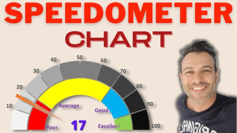
A gauge (or speedometer) chart tracks a single number against its target, with a needle that moves when the data changes. You build it from two doughnut charts and one pie chart, layered on top of each other.

1. Set up three small data tables

Categories (values in B3:B7): the size of each performance band, plus a large value for the hidden bottom half of the dial.
Labels: the scale numbers from 0 to 100 (change them if you need a different range). These sit in D3:D13.
Pointer (H3:H5): the pointer value you want to track, the thickness of the needle, and a rest value. The rest is the total of the dial minus the pointer value and the thickness, so the three always add up to the full circle.

2. Create the first doughnut

Go to Insert > Doughnut to get a blank chart. Right-click it, choose Select Data > Add, name the series Category and select B3:B7 as the values.

3. Turn it into a half circle

Right-click the chart, choose Format Data Series and set Angle of first slice to 270°. Then right-click only the bottom half, choose Format Data Point and set it to No fill. Colour the remaining four bands (the video uses red, yellow, blue and green).

4. Label the bands

Right-click the chart, choose Format Data Labels, tick Value From Cells and select the labels next to the first table.

5. Add the second doughnut for the scale

Select Data > Add again, name the series Labels and select the values column of the second table. Repeat step 3: hide the bottom half and colour the rest. For its data labels, tick Value From Cells, select D3:D13 and untick Value, otherwise every label shows the same number.

6. Build the needle

Select Data > Add a third series named Pointer with H3:H5 as the values. Excel draws it as another doughnut, so right-click and choose Change Series Chart Type and set the third series to Pie. Check its angle is 270° too. Give the two large pie slices No fill, so only the thin sliver is left. That’s your needle. To make it stand out, open Format Data Point and set Point Explosion to 5%.

7. Show the value in the middle

Go to Insert > Text Box and draw it in the centre of the gauge. With the text box selected, type = in the formula bar and click the cell that holds the pointer value. The box now updates whenever the data does. Finally, delete the legend and tidy the label positions.

Go further

My Excel Dashboard & Data Analysis Masterclass course shows you how to build 10 interactive dashboards from scratch, where gauges like this are a regular feature.