How to Create Dependent Drop-Down Lists in Excel That Update Automatically

Pick a category in one cell, and the next dropdown only shows the items that belong to it.

Choose Fruit, get apples and pears. Choose Vegetables, get carrots and onions.

In this tutorial we build dependent dropdowns in Excel using Data Validation,
Excel Tables and the INDIRECT function. Once it’s set up, adding a new item to
your list makes it appear in the dropdown automatically — no going back to adjust anything.

Watch: self-updating dependent drop-downs in 8 minutes

Prefer reading? The same steps are written out below the video.

Step-by-step

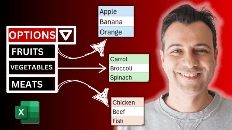
Pick a category in one cell (Fruits, Vegetables or Meats) and the next drop-down shows only that category’s items. Because the lists are Excel tables, adding a new item later makes it appear in the drop-down automatically.

1. Put the lists on their own sheet

Add a new sheet and rename it Lists. In B1 type Fruits with items below (Apple, Banana, Orange); in D1 Vegetables (Carrot, Broccoli, Spinach); in F1 Meats (Chicken, Beef, Fish). Leave an empty column between lists so they don’t run together.

2. Turn each list into a named table

Select the Fruits list including its header, go to Insert > Table and tick My table has headers. On Table Design, change the Table Name to Fruits. Do the same for Vegetables and Meats. The table names must match the category names exactly. Give each table a colour if you like.

3. Create the category drop-down

On the main sheet, select B2:B16 and go to Data > Data Validation. Set Allow to List and type the source as Fruits,Vegetables,Meats.

4. Create the dependent drop-down

Select C2 (and the cells below), open Data Validation, choose List and enter:

=INDIRECT(B2)

INDIRECT takes the text in B2, such as Fruits, and treats it as the name of a range, here the Fruits table. Because B2 has no dollar signs, each row looks at its own category cell.

5. Add items any time

Go to the Lists sheet and type a new item at the bottom of a table, for example Avocado under Fruits. The table grows by itself and the drop-down includes it straight away. Delete a table row to remove an item. No need to touch the validation again.

Go further

My Excel Tips & Shortcuts: 100+ Powerful Hacks course collects a hundred time-saving techniques like this one.