
How to Highlight the Active Row and Column in Excel (Crosshair Effect)
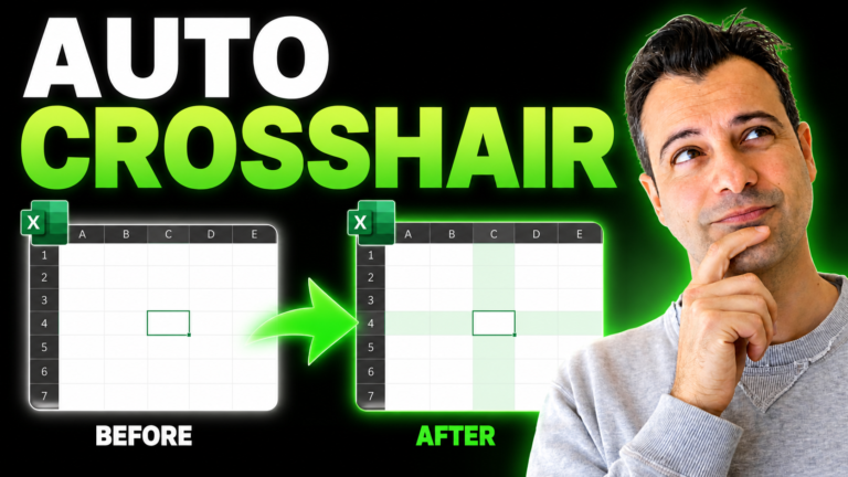
Ever get lost in a huge spreadsheet, tracing across with your finger to find the
right row?
In this tutorial we build a crosshair effect — the active row and column
highlight automatically as you move around, so you always know exactly where
you are. We start with conditional formatting, add one line of VBA to make it
update live, then build a toggle so you can switch it on and off.
Watch the full build
Prefer reading? The main steps, formulas and code are written out below the video.
Step-by-step
Clicking a row number or column letter highlights it in grey, but only one direction at a time, with no colour choice, and it’s slow on big sheets. Instead, you’ll make the active cell’s row and column light up automatically, like a crosshair, with an on/off switch and a toggle button.
1. Highlight the active row
Select your data (click A4, then Ctrl+Shift+Right Arrow and Ctrl+Shift+Down Arrow). Go to Home > Conditional Formatting > New Rule > Use a formula, enter the formula below, and pick a bright fill such as light orange:
=ROW()=CELL("row")
It’s true for every cell on the same row as the active cell. For the active column instead, use =COLUMN()=CELL("col").
2. Highlight both: the crosshair
For row and column together, use:
=OR(ROW()=CELL("row"),COLUMN()=CELL("col"))
3. Make the active cell stand out (optional)
Add one more rule with a stronger colour (bold yellow or dark green) for the cell where row and column meet:
=AND(ROW()=CELL("row"),COLUMN()=CELL("col"))
In Conditional Formatting > Manage Rules, move this rule above the crosshair rule so it takes priority.
4. Make it follow your clicks with one line of VBA
CELL(“row”) only updates when Excel recalculates, so on its own the highlight stays put until you press F9. To fix that, turn on the Developer tab (right-click the ribbon > Customize the Ribbon > tick Developer), open Visual Basic, and double-click your sheet in the Project pane. In the left drop-down choose Worksheet, in the right one SelectionChange, and add one line:
Private Sub Worksheet_SelectionChange(ByVal Target As Range)
    Target.Calculate
End Sub
Every time you select a new cell, Excel recalculates it, so the highlight jumps with you. Save as an Excel Macro-Enabled Workbook (.xlsm).
5. Add an on/off switch
In an out-of-the-way cell such as C1 (with a label like Highlight switch in B1), add a drop-down: Data > Data Validation > List, source On,Off. Name the cell Highlight_Switch in the Name Box.
Then add a new conditional formatting rule on the data with the formula below and no format:
=IF(Highlight_Switch="Off",TRUE,FALSE)
In Manage Rules, move it to the top and tick Stop If True. When the switch is Off, Excel stops before the highlight rules run.
6. Add a one-click toggle button
In the VBA editor, choose Insert > Module and add a small macro that flips the switch, for example:
Sub ToggleHighlight()
    With [Highlight_Switch]
        If .Value = "Off" Then .Value = "On" Else .Value = "Off"
    End With
End Sub
Insert a rounded rectangle shape, type Toggle highlight on it, right-click it, choose Assign Macro and pick ToggleHighlight. One click now turns the crosshair on or off.
Bonus: keep headers visible
Combine the crosshair with View > Freeze Panes (or turn the data into a table with Ctrl+T) so your headers stay in view as you scroll.
Go further
My Excel Macros & VBA Programming for Beginners course takes you from one-line macros like these to writing your own VBA, with no prior coding needed.
No matter your profession, stop wasting precious hours crunching numbers.
Get the Excel training that builds an unbeatable resume and warp drives your career.