
THE CHART PACK
Mekko, fan chart, bullet, gauge, waterfall — the ones Excel won’t build for you. All finished and working. Free, instant, yours to keep.
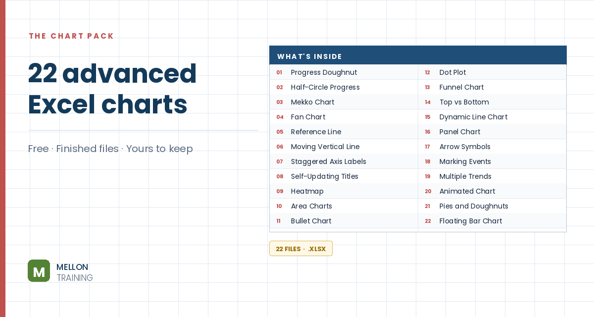
What’s in the pack
Free, instant, and yours to keep.
No spam, ever. Unsubscribe with one click.
One practical Excel tip a week.
Watch the 8-minute video or follow the written steps below. A finished waterfall chart is included in the free chart pack above.
A waterfall (or bridge) chart shows how a starting value is built up or worn down by a series of positive and negative changes. The first and last columns are totals, and the floating columns in between show each rise or fall. It’s ideal for monthly cash flow, sales analysis or product earnings.
Start with a start value and the sales change for each month (some up, some down), followed by an end row. Add three helper columns: Base (B), Negative (C) and Positive (D), with the monthly change in column E.
The negative column shows falls as positive numbers, and the positive column shows rises. One way to write them, in row 5:
=IF(E5<=0,-E5,0)=IF(E5>=0,E5,0)Copy both down the table.
Each floating column sits on an invisible base. In B6:
=B5+D5-C6
Copy it down, including the end row.
Select A4:D18 (leaving out the sales-change column) and go to Insert > Column Chart > Stacked Column.
Click the Base series, right-click and choose Format Data Series. Under Fill & Line, set No fill and No line. Delete Base from the legend. It now looks like a waterfall chart.
Select a series and go to Chart Design > Add Chart Element > Data Labels > Center. Delete any zero labels and format the rest. Your waterfall chart is ready.
YOUR NEXT STEP
Almost every “how did they build that” chart is the same idea — a helper column feeding an invisible series. Once you spot the pattern you stop needing tutorials. You look at a chart and think “that’s two series stacked, one of them hidden”, and you’re usually right.
30-day money-back guarantee, handled by Udemy. No forms, no questions.
★★★★★ Join 80,000+ students
Andreas Exadaktylos · Microsoft-certified Excel instructor · mellontraining.com
WATCHING ON YOUTUBE?
11 step-by-step courses on Excel, Power BI, Python and AI, all on Udemy with lifetime access.