
THE DASHBOARD PACK
Kanban board, habit tracker, KPI report, search bar and more — built, working, ready to take apart. Free, instant, yours to keep.
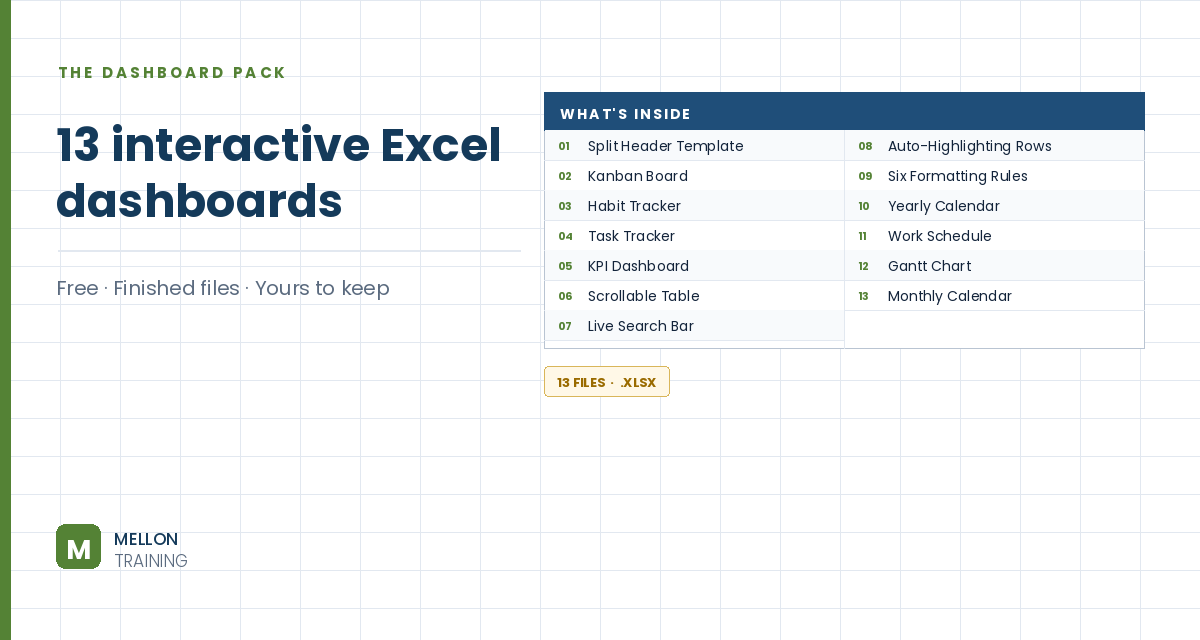
What’s in the pack
Free, instant, and yours to keep.
No spam, ever. Unsubscribe with one click.
One practical Excel tip a week.
Watch the 5-minute video or follow the written steps below. The free dashboard pack above has finished dashboards that use these filters.
Slicers and timelines are Excel’s two visual filter tools, and you’ll find them in almost every good dashboard. Slicers filter by categories (such as country or product) with a click, and a timeline filters by dates. The example dashboard already has PivotTables and PivotCharts built from the workbook’s Data Model.
Go to Insert > Timeline. Excel asks which data to connect to: open the Data Model tab, choose This Workbook Data Model and click Open. Tick the date field (Order Date in the example) and click OK. Move the timeline under the PivotTable it belongs with.
With the timeline selected, pick a style from the Timeline (Options) tab. Then the important step: click Report Connections and tick every PivotTable and PivotChart you want it to control. Otherwise it filters only one of them.
Test it: switch the timeline between years, quarters and months, and drag across a range of dates. The connected reports update instantly.
Go to Insert > Slicer, connect to the workbook Data Model the same way, and tick the fields you want to filter by. The example uses Country and Product Category. Move the slicers into place and choose a style from the Slicer (Options) tab.
Don’t skip this: right-click each slicer (or use the Slicer tab), choose Report Connections and tick all the PivotTables and charts, so one click filters the whole dashboard.
Add clear titles above the charts (the example uses Sales per Product Category and Sales per Quarter) and format them. Finally, click through the slicers and timeline and check that every value changes as expected.
YOUR NEXT STEP
Every dashboard in this pack rests on the same three techniques: conditional formatting, data validation and dynamic formulas. Learn those properly and you stop collecting templates — you build whatever the job actually needs.
30-day money-back guarantee, handled by Udemy. No forms, no questions.
★★★★★ Join 80,000+ students
Andreas Exadaktylos · Microsoft-certified Excel instructor · mellontraining.com
WATCHING ON YOUTUBE?
11 step-by-step courses on Excel, Power BI, Python and AI, all on Udemy with lifetime access.